Other useful functions

Abstract

This section covers the capability of plasmoRUtils to carry out other mundane bioinformatics tasks.

Introduction

Other than search functions, the plasmoRUtils package offers various other functions that are routinely needed when performing bioinformatics analysis. Their usage is discussed below.

With release 71 of VEuPathDB, only users with subscription and API key can access the database programmatically. Use usethis::edit_r_environ(scope = "user") to add VEuPathDB API using VEUPATHDB_API_KEY variable. By default, all the functions look for VEUPATHDB_API_KEY variable for API key. Should you store your key using any other variable, supply it using api_key argument in VEuPathDB associated functions.

# Load package and some other useful packages by using
suppressPackageStartupMessages(
  suppressWarnings({
    library(plasmoRUtils)
    library(dplyr)
    library(tibble)}))

Making OrgDb and TxDb objects

For a non-model organism, functions such as clusterProfiler::enrichGO() require an appropriate OrgDb annotation package. Unfortunately, this requires ability to understand and use AnnotationDbi package. To make development of such packages quickly, we wrote a wrapper function that instantly creates a TAR file that can be used and shared by the user in no time.

## List organism you are interested in making org.db package from VEuPathDB.
## Use the links from PlasmoDB directly or provide locally saved GFF and GAF files.

## Get the taxonomy ID using listVeupathdb(customFields = c("primary_key", "ncbi_tax_id"))

# easymakeOrgdb() itself supports authenticated HTTPS URLs.
# No extra temporary-file downloader is necessary.
archive <- easymakeOrgdb( 
  gff = "https://plasmodb.org/a/service/raw-files/release-71/Pfalciparum3D7/gff/data/PlasmoDB-71_Pfalciparum3D7.gff",
  gaf = "https://plasmodb.org/a/service/raw-files/release-71/Pfalciparum3D7/gaf/PlasmoDB-71_Pfalciparum3D7_GO.gaf",
  out.dir = "./annotation", taxid = 36329,
  genus = "Plasmodium", sp = "falciparum3D7", version = "0.1.0",
  maintainer = "Jane Doe <jane@example.org>",
  api_key = Sys.getenv("VEUPATHDB_API_KEY"),
  overwrite = TRUE
)
install.packages(archive, repos = NULL, type = "source")

## Once the package is ready, one can use clusterProfiler as follows

library(clusterProfiler)
library(org.Pfalciparum3D7.eg.db)


genes <- c("PF3D7_0102200", "PF3D7_0207400")
bkg_genes <- AnnotationDbi::keys(org.Pfalciparum3D7.eg.db, keytype = "GID") # replace with all genes eligible in your assay
ego <- enrichGO(gene          = genes,
                universe      = bkg_genes,
                OrgDb         = org.Pfalciparum3D7.eg.db,
                keyType = "GID",
                ont           = "BP",
                minGSSize=3,
                pAdjustMethod = "BH",
                pvalueCutoff  = 0.05,
                qvalueCutoff  = 0.05,
        readable      = FALSE)

The function above will create an org.db tar file which can be installed and loaded to be used with clusterProfiler.

Similarly, if users want to make TxDb object in R to use other R packages such as gDNAx used to access the genomic DNA contamination, they can do so easily using easyTxDbmaker() function.

txdb <- easyTxDbmaker(
 gff="ToxoDB-71_TgondiiME49.gff",
 fasta="ToxoDB-71_TgondiiME49_Genome.fasta",
 abbr="TgondiiME49",
 taxid=508771,org = "Toxoplasma gondii ME49",
 db = "ToxoDB release 68")

Other easy functions

Users are also provided with easy functions which are wrapper functions around routinely used to analyze bioinformatics data.

TPM normalization and visualization

In this section we will see how we can calculate effective gene lengths from a GFF file followed by TPM normalization and visualize the resulting normalized matrix. These functions are provided since most of the RNASeq data present on VEuPathDb is TPM normalized and therefore make it easy to plot the database procured values alongside your own samples.


# To calculate the effective length of the genes you can use the following function. Adding extra layer 
# of code to fetch the GFF directly from database
getEffLenVEuPath <- function(
    url,
    api_key = Sys.getenv("VEUPATHDB_API_KEY"),
    timeout = 60
) {

  if (!nzchar(api_key)) {
    stop(
      "VEuPathDB API key is missing.",
      call. = FALSE
    )
  }

  tmp <- tempfile(fileext = ".gff")
  on.exit(unlink(tmp), add = TRUE)

  httr2::request(url) |>
    httr2::req_auth_bearer_token(api_key) |>
    httr2::req_timeout(timeout) |>
    httr2::req_perform(path = tmp)

  getEffLen(tmp)
}

getEffLenVEuPath(
  "https://plasmodb.org/a/service/raw-files/release-71/Pfalciparum3D7/gff/data/PlasmoDB-71_Pfalciparum3D7.gff"
) |>
  head()
#> # A tibble: 6 × 2
#>   GeneID        Length
#>   <chr>          <dbl>
#> 1 PF3D7_0100100   6492
#> 2 PF3D7_0100200    996
#> 3 PF3D7_0100300   3984
#> 4 PF3D7_0100400   1119
#> 5 PF3D7_0100500    112
#> 6 PF3D7_0100600   1080

The above function returns a dataframe which can be fed to the easyTPM() function alongside the count matrix. The output retains matched gene lengths as its final column. TPM cannot be converted back to the original raw counts from TPM and gene length alone because the original library scaling factor is not retained. This is also helpful since the exon-intron boundaries are always evolving as the new data-sets become available.

library(ggplot2)
## Generating dummy effective length for a local demonstration
gene_info <- data.frame(GeneID = c("PF3D7_0100100", "PF3D7_0100200", "PF3D7_0100300"), Length = c(6492, 996, 3984))

## Making a dummy count matrix
count_matrix <- matrix(c(10, 20, 30, 40, 50, 60),
                       nrow = 3, ncol = 2,
                       dimnames = list(c("PF3D7_0100100", "PF3D7_0100200", "PF3D7_0100300"), c("sample1", "sample2"))
                       )

## TPM normalization
test <- easyTPM(count_matrix, gene_info) %>% rownames_to_column(var = "GeneID")

## TPM visualization as a bubble plot
df <- reshape2::melt(test[, -ncol(test)], id.vars = "GeneID", na.rm = TRUE) 
easyExpPlot(df,x="variable",y="GeneID",value="value", type = "bubble")+labs(x="Samples",y="Gene IDs")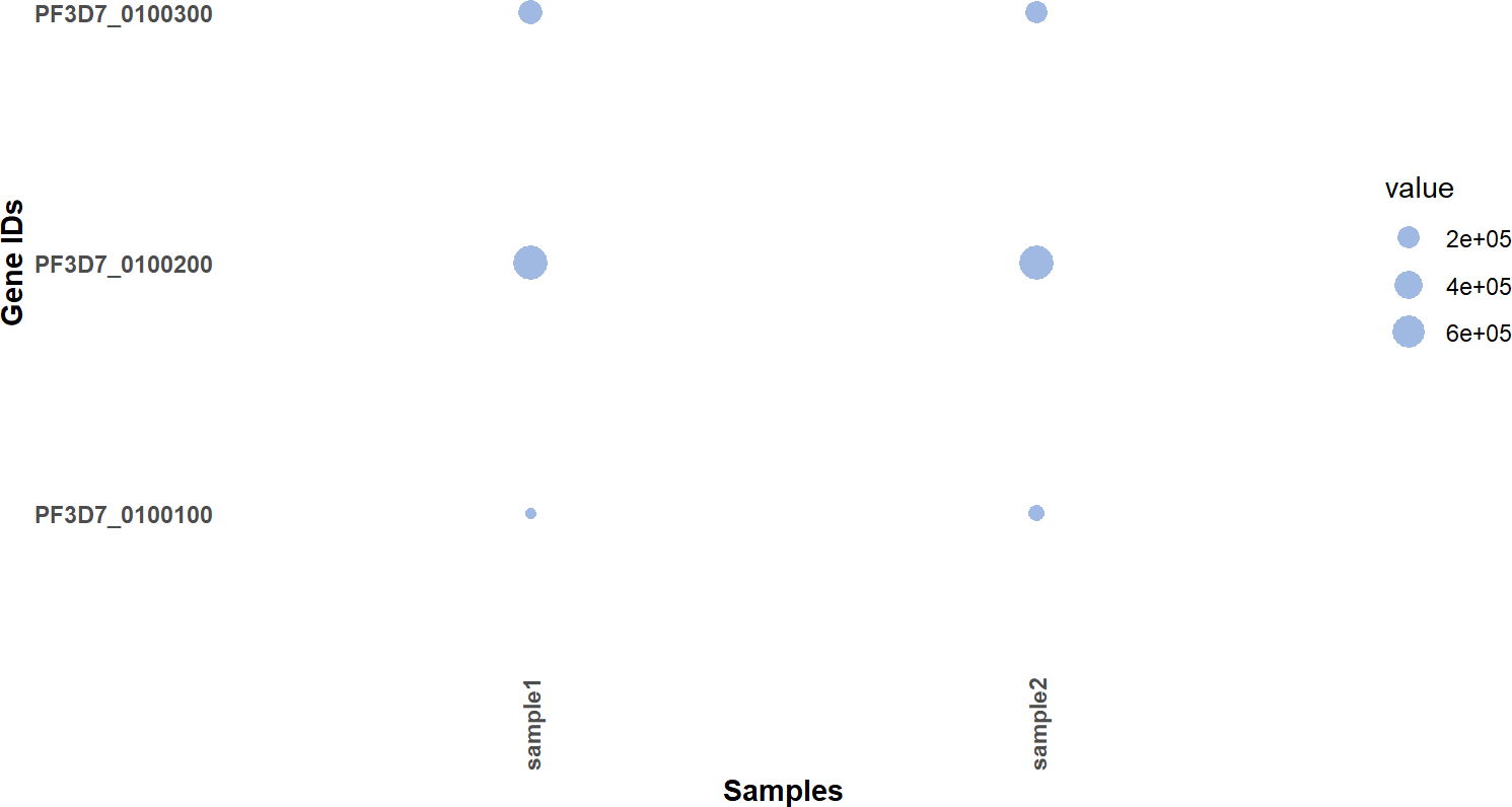

You can also plot normalized expression data as line plot if you have cluster of genes with similar pattern of expression. To demonstrate this we will use a subset of genes from (Subudhi et al. 2020) time series dataset. We will perform TPM normalization, followed by log transformation and eventually use the Z-scores for visualization.


data("subudhi2020")
count_matrix <- SummarizedExperiment::assay(subudhi2020, "counts") %>% as.matrix()
gene_info <- getEffLenVEuPath(
  "https://plasmodb.org/a/service/raw-files/release-71/Pfalciparum3D7/gff/data/PlasmoDB-71_Pfalciparum3D7.gff"
)

# easyTPM() requires a length for every row.
missing_lengths <- setdiff(rownames(count_matrix), gene_info$GeneID)
if (length(missing_lengths)) stop("Missing exon-union lengths for ", length(missing_lengths),
                                  " count-matrix genes; reconcile the annotation release.")
normalised <- easyTPM(count_matrix, gene_info) 

## Since normalized matrix have effective gene length column at the end
logTransformed <- log2(as.matrix(normalised[, -ncol(normalised), drop = FALSE]) + 1)

## Get z-scores
# invariant genes have undefined standardized scores; retain NA for these rows.
z.mat <- t(scale(t(logTransformed), scale = TRUE, center = TRUE)) %>% # per-gene Z-scores
  as.data.frame() %>% tibble::rownames_to_column(var = "GeneID") 

## Subsetting few genes of interest
gois <- c("PF3D7_1476300","PF3D7_0220800","PF3D7_0936200","PF3D7_0402200","PF3D7_1401600","PF3D7_0831600","PF3D7_0204100","PF3D7_1458300","PF3D7_0935800","PF3D7_0929400","PF3D7_1439000","PF3D7_0905400","PF3D7_1334600","PF3D7_1121300","PF3D7_0302500","PF3D7_1232800","PF3D7_0310400","PF3D7_1001600")

## Transforming data frame for visualisation
df <- z.mat %>% 
  subset(.,GeneID %in% gois) %>% 
  reshape2::melt(., id.vars = "GeneID", na.rm = TRUE)

easyExpPlot(df,x="variable",y="value",value="GeneID")+
  labs(y="Z-scores",x="Samples")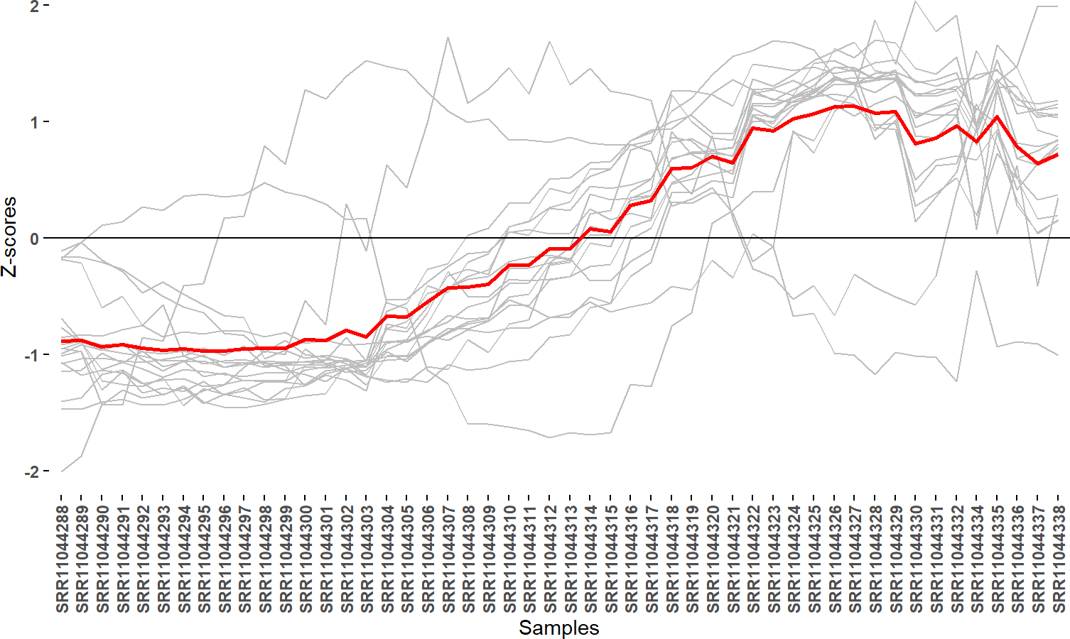

easyExpPlot() can be used to plot expression values obtained from any kind of applied normalization and transformation.

Support for NOISeq `readData` function for non-model organism

When using NOISeq for QC, users are often required to provide various information alongside count matrices. These information includes biotype, chromosome, gc content, length of the features etc. These arguments are listed as optional but are required by NOISeq package for making QC plots. To enable users to get these information from the same reference FASTA file and GFF file used by user for alignment, we wrote easyNOISeqAnnot() function that enable users to quickly get this information from GTF/GFF file and FASTA file and return a data frame. These can be provided as a URL or as locally stored files.

gene_info <- easyNOISeqAnnot(
 gff="ToxoDB-71_EpraecoxHoughton.gff",
 fasta = "ToxoDB-71_EpraecoxHoughton_Genome.fasta",
 name = "EpraecoxHoughton")

gene_info %>% head()

You can now pass the data frame contents to NOISeq::readData() function as follows.

data_NOISEQ <- NOISeq::readData(data = counts,
                        length=setNames(gene_info$length, gene_info$gene_id),
                        gc=setNames(gene_info$gc, gene_info$gene_id),
                        biotype=setNames(gene_info$gene_biotype, gene_info$gene_id),
                        chromosome = gene_info[,c("chr","starts","ends")],
                        factors = meta)

Check synchronization of Bulk RNASeq samples using `easyLabelTransfer()`

easyLabelTransfer() is a wrapper function written around SingleR SingleR() function to quickly use count matrices from Bulk/ Single cell Reference data sets to check synchronization (time point and stage) of the Parasite Bulk RNASeq samples and can be used for QC purposes.

Here, for demonstration purpose, we will use single cell RNASeq data from Malaria Cell Atlas and use (Subudhi et al. 2020) Bulk time-series dataset to transfer labels and see the distribution of the cells across different time points.

Other data sets provided with the package includes:

Reanalyzed time course asexual Microarray dataset of P. falciparum 3D7 from (Painter et al. 2018): data("painter2018")
Reanalyzed time course asexual Bulk RNASeq (Single-end) of P. falciparum 3D7 from (Toenhake et al. 2018): data("toenhake2018")
Reanalyzed time course asexual Bulk RNASeq (Paired-end) of P. falciparum 3D7 from (Kucharski et al. 2020): data("kucharski2020")
Reanalyzed scRNAseq of T. gondii ME49 data from (Lou et al. 2024): data("gubbels2024")
Reanalyzed scRNAseq of T. gondii ME49 data from (Xue et al. 2020): data("boothroyd2020")
Reanalyzed asexual Bulk RNASeq (Paired-end) of P. falciparum 3D7 from (Wichers et al. 2019): data("wichers2019")
Reanalyzed time course gametocytes Bulk RNASeq (Paired-end) of P. falciparum 3D7 from (Jeninga et al. 2023): data("petter2023")

Next, Malaria cell atlas (MCA) is a database comprising of single cell data sets and can be accessed using the following functions.

listMCA() function enables you to filter and list scRNASeq data sets for which data download links are available. User can use this function to view a table to metadata about the dataset or download these datasets recursively rather than manually downloading single dataset at a time.
easyMCA() enables users to import the count matrix and metadata directly in the R environment directly. Written mainly for pipeline development.

Now, lets use the function enlisted above alongside easyLabelTransfer() as shown below.

Note: easyLabelTransfer() returns a SingleR results object (typically a DFrame), which can be used with SingleR plotting functions.

library(SingleR)
set.seed(12458)
## Fetching the URL
mcalist <- listMCA()
data("subudhi2020") ## reference dataset
subudhi2020 <- subudhi2020[,1:42] ## Skipping samples after 43 Hpi since they highly correlate with 43hpi itself.

## Using this reference set
url <- "https://www.malariacellatlas.org/downloads/pf-ch10x-set4-biorxiv.zip"

raw_counts <- easyMCA(url,type = "raw")
rownames(raw_counts) <- gsub("-","_",rownames(raw_counts))
meta <- easyMCA(url,type="data")

## Retaining only Asexual stage cells and Lab isolates.
meta <- subset(meta, meta$STAGE_LR %in% c("ring","trophozoite","schizont") & DAY != "Field")
stopifnot(all(rownames(meta) %in% colnames(raw_counts))) 
raw_counts <- as.matrix(raw_counts[, rownames(meta), drop = FALSE]) 
storage.mode(raw_counts) <- "numeric" 

## Filtering away field isolates and sexual stage cells

labels <- easyLabelTransfer(queryCounts = raw_counts,
                            refCounts = SummarizedExperiment::assay(subudhi2020, "counts"), 
                            referenceMeta = as.data.frame(SummarizedExperiment::colData(subudhi2020)),
                            labelCol = "timetag", 
                            isrefBulk = TRUE, 
                            de.n=200,
                            fine.tune=TRUE) 

table(labels$pruned.labels)
#> 
#> 11hpi 13hpi 15hpi 17hpi 19hpi 21hpi 23hpi 25hpi 29hpi 33hpi 37hpi 39hpi  3hpi 
#>   831   508   381   593    38  2592    19  3678  2836  3148   150  2037  2897 
#> 41hpi 43hpi  5hpi  7hpi  9hpi 
#>  2017  5505   731   229   307

df <- as.data.frame(table(labels$labels), stringsAsFactors = FALSE) 
names(df) <- c("Timepoint", "Freq") 
levels_order <- unique(as.character(subudhi2020$timetag)) 
df$Timepoint <- factor(df$Timepoint, levels = levels_order) 

ggplot2::ggplot(df, ggplot2::aes(x = Timepoint, y = Freq)) +
  ggplot2::geom_col(fill = "#2595be") +
  ggplot2::geom_text(ggplot2::aes(label = Freq), vjust = -0.2) +
  ggplot2::labs(x = "Time points", y = "Number of cells") +
  ggplot2::theme_minimal() +
  ggplot2::theme(axis.text.x = ggplot2::element_text(angle = 90, vjust = 0.5))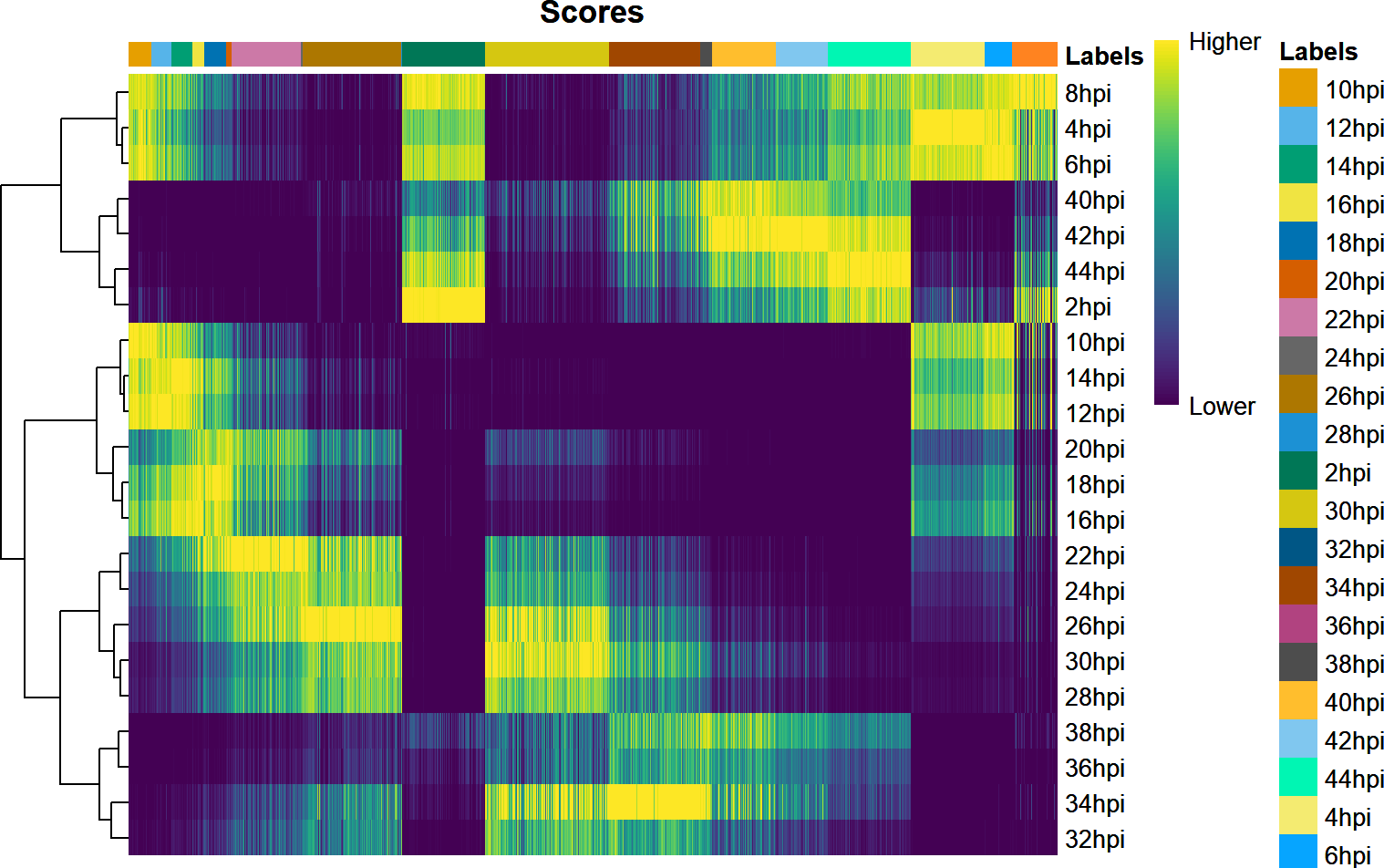


SingleR::plotScoreHeatmap(labels, show_colnames = FALSE,
                           show.pruned = FALSE, cluster_cols = FALSE,
                           cluster_rows = FALSE, rows.order = levels_order)

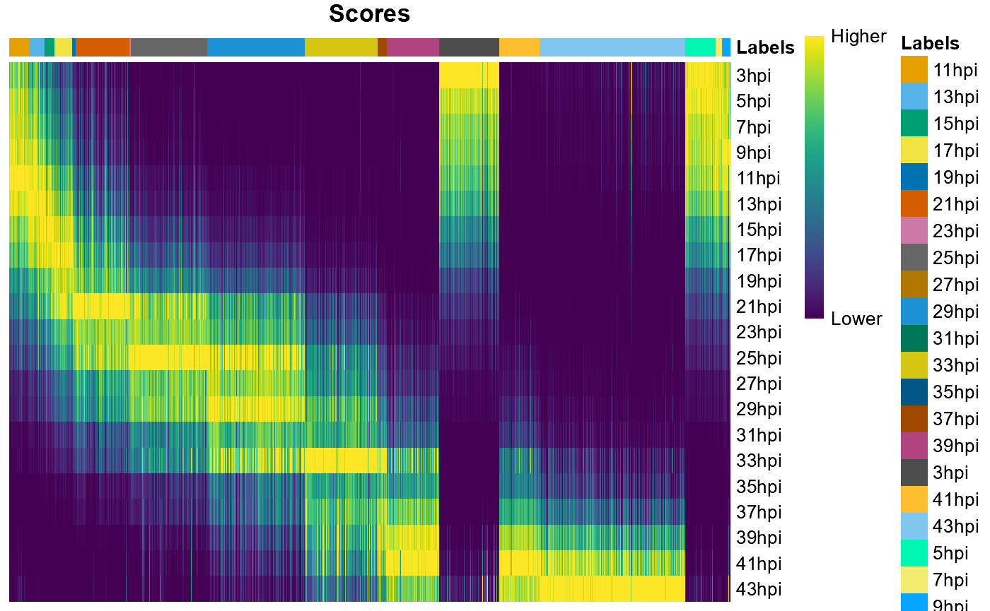
You can see that cells from some time points are underrepresented in our Malaria Cell Atlas.

GO Enrichment using `easytopGO()`

VEuPathDB constituent database allow users to perform GO Enrichment analysis. However, there is no option to set the background genes and by default all the genes in the are used. This is not an ideal approach. Moreover, since Gene Ontologies are curated using different pipelines by different enrichment providers, the results might differ just based on source of Ontologies. Similarly the Ontology data might not be available in other databases such as BioMart and you would like to use custom GAF file.

Users of parasite domain might wish to use GAF files provided by VEuPathDB constituent database and of specific genome assembly as per their hypothesis. To enable users to do that, GO enrichment analysis can be performed easily and quickly using our easytopGO() wrapper function. For Fisher testing, supply a uniquely named numeric vector of gene-level p-values (or adjusted p-values) for the selected genes, with gene IDs as names. The full eligible-gene universe must be supplied through bkggset. For KS testing, supply genuine gene-level p-values for every background gene. weight01 remains the package default; choose algo = "classic" for conventional, ShinyGO-style Fisher ORA. Finally users can use gaf argument to supply .gaf file obtained from VEuPathDBs constituent database of interest.

For well known organisms, Biomart Ontologies can also be used. In such case user has to provide mart argument and figure out key for Ensembl gene IDs . However, many times the parasite assemblies used as reference by Ensembl might not match with parasite assembly used by VEuPathDB. In such cases there might be mismatches between gene IDs (see one such issue here).

You can also change category argument to specify which GO category you want to test enrichment for. Since for most of the parasites, sub-cellular localization and Molecular function information is sparingly available, “BP” has been set as the default.

Results already generated by another enrichment tool are not valid geneID input to easytopGO(): supply gene-level scores for the selected genes and an explicit eligible-gene universe instead.

library(topGO)
# Making a named numeric vector of adjusted gene-level p-values (selected genes only).
gois <- c("PF3D7_0102200","PF3D7_0207400","PF3D7_0207500","PF3D7_0207600","PF3D7_0207700","PF3D7_0207800","PF3D7_0207900","PF3D7_0208000","PF3D7_0404700","PF3D7_0501500","PF3D7_0502400","PF3D7_0618000","PF3D7_0731800","PF3D7_0930300","PF3D7_1116000","PF3D7_1247800","PF3D7_1334700")


p_values <- c(1.767929e-49,3.886063e-148,6.459285e-269,0.000000e+00,6.842121e-132,
5.282318e-178,1.140221e-224,1.625665e-100,6.177129e-08,1.484155e-03,2.789648e-10,2.300720e-12,7.450697e-30,3.417972e-89,4.846689e-73,1.207966e-11,4.173777e-51)
names(p_values) <- gois

## Using all genes captured as a background

background.gset <- rownames(SummarizedExperiment::assay(subudhi2020, "counts"))
stopifnot(all(names(p_values) %in% background.gset)) #selected genes must belong to the background

easytopGOVEuPath <- function(
    gaf,
    api_key = Sys.getenv("VEUPATHDB_API_KEY"),
    timeout = 60,
    ...
) {
  if (!nzchar(api_key)) stop("VEuPathDB API key is missing.") 
  gaf_tmp <- tempfile(fileext = ".gaf")

  # Clean up after function finishes
  on.exit(
    unlink(c(gaf_tmp)),
    add = TRUE
  )

  # Download GAF
  httr2::request(gaf) |>
    httr2::req_auth_bearer_token(api_key) |>
    httr2::req_timeout(timeout) |>
    httr2::req_perform(path = gaf_tmp)

  # Pass the locally downloaded GAF to easytopGO()
  easytopGO(geneID = p_values,
            useGAF = TRUE,
            useBiomart = FALSE,
            gaf=gaf_tmp,
            bkggset = background.gset, 
            category = "BP", stats = "fisher",
            algo = "classic", fdr = TRUE, correction = "BH", ...) 
}


## Performing ORA
gores<- easytopGOVEuPath(gaf = "https://plasmodb.org/a/service/raw-files/release-71/Pfalciparum3D7/gaf/PlasmoDB-71_Pfalciparum3D7_GO.gaf")

## Plotting the results. 
goplt <- easyGOPlot(gores, title = "GO Biological processes", limit = 20, sortby = "padj")
goplt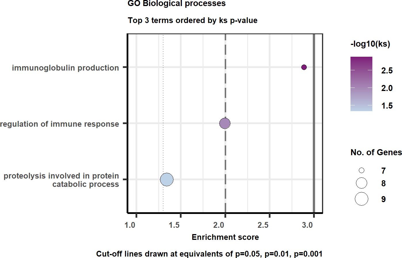


## Making circular plot
goplt + ggplot2::theme_minimal() + ggplot2::coord_polar() + ggplot2::ylab("")

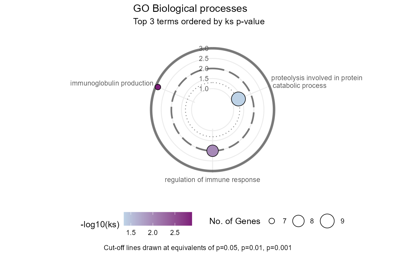
easyGOPlot() is an adapted and modified version of what has been provided by Kevin Blighe on Biostars. You can use limit argument to limit number of terms to be plotted.easytopGO() also enables users to use Org.db package if available for your organism of interest. An examplary code is given below

library(org.Pfalciparum3D7.eg.db)
pfdb <- org.Pfalciparum3D7.eg.db

## res is the result obtained from DESeq2
res <- ggVolcano::add_regulate(res, log2FC_name = "log2FoldChange",
             fdr_name = "padj",log2FC = 1, fdr = 0.05)
res <- res[!duplicated(res$`Gene ID`),] ## ensuring only one entry of gene duplicates is retained


ok <- !is.na(res$padj) & !is.na(res$`Gene ID`)
background.gset <- res$`Gene ID`[ok]
down <- ok & !is.na(res$log2FoldChange) &
  res$regulate == "Up"
geneList <- stats::setNames(res$padj[down], res$`Gene ID`[down]) 

gores.fisher <- easytopGO(
  geneID = geneList, 
  bkggset = background.gset,
  algo = "classic",
  OrgDb = pfdb, orgdb_keytype = "GID", 
  useBiomart = FALSE, useGAF = FALSE,
  stats = "fisher", category = "BP", 
  fdr = TRUE, correction = "BH"
)

When using Fisher (perform on Upregs and Downregs separately), you answer the following question: “Is the proportion of significant genes (up or down regulated genes) inside this specific GO term significantly higher than the proportion of significant genes across the rest of the genome?”

When using KS, you answer the following question: “Do the genes belonging to this specific GO term lay toward the very top of my p-value ranking compared to a random distribution?”. However, if you split the genes into categories such as genesets with positive fold change and negative foldchange, your question would be “Which GO terms have stronger differential-expression signals among positively/negatively changing genes?”

## Examplary code to use KS

# Retain eligible genes with positive fold changes
# Exclude missing adjusted p-values
ok.up <- !is.na(res$`Gene ID`) &
  nzchar(as.character(res$`Gene ID`)) &
  !is.na(res$log2FoldChange) &
  res$log2FoldChange > 0 &
  !is.na(res$padj) &
  !is.na(res$pvalue) &
  is.finite(res$pvalue) &
  res$pvalue >= 0 &
  res$pvalue <= 1

up_universe <- res[ok.up, , drop = FALSE]

# Using genuine raw p-values as continuous KS scores because we are using a continuous ranking statistic. BH-adjusted p-values can also be used, but adjustment may introduce extra ties and change the ranking.
up_ks_vector <- stats::setNames(
  up_universe$pvalue,
  as.character(up_universe$`Gene ID`)
)

# Use exactly the same genes as the KS background
up_background <- names(up_ks_vector)

# Perform KS enrichment
gores.ks.up <- easytopGO(
  geneID = up_ks_vector,
  bkggset = up_background,
  algo = "classic",
  gaf = "PlasmoDB-71_Pfalciparum3D7_GO.gaf",
  useBiomart = FALSE,
  useGAF = TRUE,
  stats = "ks",
  category = "BP",
  fdr = TRUE,
  correction = "BH"
) # Which GO terms have stronger differential-expression signals among positively/negatively changing genes

Screening the Signal Peptides from PDBs

We also offer a convenient function, easyAF2Signal(), to diagnose potential false-positive signal peptides using SignalP predictions from the VEuPathDB database and AlphaFold2 structures, based on an observational study conducted by (Sanaboyana and Elcock 2024). The authors found that putative N-terminal signal-peptide regions (often approximately 20–30 amino acids) are typically disengaged from the protein body and lack atomic contacts, and AlphaFold2 attempts to model them in a similar way.

easyAF2Signal() is an R equivalent with slight modifications to the Fortran code provided by the authors, which reports additional information, such as the number of residues remaining after pLDDT filtering.

We did this modification because, if all the signal peptide residues have low pLDDT scores and are filtered out, no residues will remain to calculate contacts with the protein body, resulting in zero contacts. This could give a false impression that the first 25 amino acids are signal peptides, but it cannot be confirmed, as the zero-contact observed is due to no residues remaining after filtering, not because the signal peptide was disengaged from the protein body.

easyAF2Signal("https://alphafold.ebi.ac.uk/files/AF-A0A140KXW6-F1-model_v6.pdb")
#>                        Name length_signalpeptide length_protein
#> 1 AF-A0A140KXW6-F1-model_v6                   25            410
#>   postbfacFiltered_signalP_res medianSignalP_bfac clevagesite_bfac
#> 1                           16              92.19            94.25
#>   postbfacFiltered_rest_res medianRest_bfac res_res_conts atm_atm_conts
#> 1                       284           93.91            65           242

In the example above, we see that signal peptide has low mean pLDDT score and therefore there are no residues left post filtering of bad quality residues leading to zero residue-residue counts res_res_conts. Thus a zero-contact result caused by filtering out all residues is inconclusive, not evidence of a signal peptide.

Session Info

utils::sessionInfo()
#> R version 4.4.1 (2024-06-14 ucrt)
#> Platform: x86_64-w64-mingw32/x64
#> Running under: Windows 11 x64 (build 26200)
#> 
#> Matrix products: default
#> 
#> 
#> locale:
#> [1] LC_COLLATE=English_India.utf8  LC_CTYPE=English_India.utf8   
#> [3] LC_MONETARY=English_India.utf8 LC_NUMERIC=C                  
#> [5] LC_TIME=English_India.utf8    
#> 
#> time zone: Asia/Riyadh
#> tzcode source: internal
#> 
#> attached base packages:
#> [1] stats4    stats     graphics  grDevices utils     datasets  methods  
#> [8] base     
#> 
#> other attached packages:
#>  [1] topGO_2.56.0                SparseM_1.84-2             
#>  [3] GO.db_3.23.1                AnnotationDbi_1.74.0       
#>  [5] graph_1.82.0                SingleR_2.6.0              
#>  [7] SummarizedExperiment_1.34.0 Biobase_2.64.0             
#>  [9] GenomicRanges_1.56.2        GenomeInfoDb_1.40.1        
#> [11] IRanges_2.38.1              S4Vectors_0.42.1           
#> [13] BiocGenerics_0.50.0         MatrixGenerics_1.16.0      
#> [15] matrixStats_1.5.0           ggplot2_4.0.3              
#> [17] tibble_3.3.1                dplyr_1.2.1                
#> [19] plasmoRUtils_1.1.3          rlang_1.3.0                
#> [21] readr_2.2.0                 janitor_2.2.1              
#> [23] BiocStyle_2.32.1           
#> 
#> loaded via a namespace (and not attached):
#>   [1] segmented_2.2-2             fs_2.1.0                   
#>   [3] ProtGenerics_1.36.0         bitops_1.1-0               
#>   [5] lubridate_1.9.5             pRoloc_1.44.1              
#>   [7] httr_1.4.9                  RColorBrewer_1.1-3         
#>   [9] doParallel_1.0.17           tools_4.4.1                
#>  [11] MSnbase_2.30.1              utf8_1.2.6                 
#>  [13] R6_2.6.1                    lazyeval_0.2.3             
#>  [15] withr_3.0.3                 prettyunits_1.2.0          
#>  [17] gridExtra_2.3.1             preprocessCore_1.66.0      
#>  [19] cli_3.6.6                   textshaping_1.0.5          
#>  [21] gt_1.4.0                    labeling_0.4.3             
#>  [23] sass_0.4.10                 mvtnorm_1.4-2              
#>  [25] S7_0.2.2                    randomForest_4.7-1.2       
#>  [27] proxy_0.4-29                pkgdown_2.2.1              
#>  [29] Rsamtools_2.20.0            systemfonts_1.3.2          
#>  [31] txdbmaker_1.0.1             AnnotationForge_1.46.0     
#>  [33] dichromat_2.0-1             parallelly_1.48.0          
#>  [35] limma_3.60.6                rstudioapi_0.19.0          
#>  [37] impute_1.78.0               RSQLite_3.53.3             
#>  [39] FNN_1.1.4.1                 generics_0.1.4             
#>  [41] BiocIO_1.14.0               gtools_3.9.5               
#>  [43] vroom_1.7.1                 dendextend_1.19.1          
#>  [45] Matrix_1.7-6                MALDIquant_1.22.3          
#>  [47] abind_1.4-8                 lifecycle_1.0.5            
#>  [49] yaml_2.3.12                 snakecase_0.11.1           
#>  [51] recipes_1.4.0               SparseArray_1.4.8          
#>  [53] BiocFileCache_2.12.0        grid_4.4.1                 
#>  [55] blob_1.3.0                  promises_1.5.0             
#>  [57] crayon_1.5.3                PSMatch_1.8.0              
#>  [59] lattice_0.23-1              beachmat_2.20.0            
#>  [61] annotate_1.82.0             GenomicFeatures_1.56.0     
#>  [63] chromote_0.5.1              mzR_2.38.0                 
#>  [65] KEGGREST_1.44.1             pillar_1.11.1              
#>  [67] knitr_1.52                  rjson_0.2.23               
#>  [69] lpSolve_5.6.23              future.apply_1.21.0        
#>  [71] codetools_0.2-20            mgsub_2.0.0                
#>  [73] glue_1.8.1                  pcaMethods_1.96.0          
#>  [75] data.table_1.18.6.1         MultiAssayExperiment_1.30.3
#>  [77] vctrs_0.7.3                 png_0.1-9                  
#>  [79] gtable_0.3.6                kernlab_0.9-33             
#>  [81] cachem_1.1.0                gower_1.0.2                
#>  [83] xfun_0.62                   prodlim_2026.03.11         
#>  [85] S4Arrays_1.4.1              coda_0.19-4.1              
#>  [87] survival_3.8-12             ncdf4_1.24                 
#>  [89] timeDate_4052.112           SingleCellExperiment_1.26.0
#>  [91] pheatmap_1.0.13             iterators_1.0.14           
#>  [93] hardhat_1.4.3               lava_1.9.3                 
#>  [95] statmod_1.5.2               MLInterfaces_1.84.0        
#>  [97] ipred_0.9-16                nlme_3.1-171               
#>  [99] bit64_4.8.6                 progress_1.2.3             
#> [101] filelock_1.0.3              LaplacesDemon_16.1.8       
#> [103] bslib_0.12.0                affyio_1.74.0              
#> [105] irlba_2.4.1                 rpart_4.1.27               
#> [107] otel_0.2.0                  colorspace_2.1-4           
#> [109] DBI_1.3.0                   nnet_7.3-21                
#> [111] tidyselect_1.2.1            processx_3.9.0             
#> [113] bit_4.6.0                   compiler_4.4.1             
#> [115] curl_8.1.0                  rvest_1.0.5                
#> [117] httr2_1.3.0                 xml2_1.6.0                 
#> [119] desc_1.4.3                  DelayedArray_0.30.1        
#> [121] plotly_4.12.1               bookdown_0.48              
#> [123] rtracklayer_1.64.0          scales_1.4.0               
#> [125] hexbin_1.28.6               affy_1.82.0                
#> [127] rappdirs_0.3.4              stringr_1.6.0              
#> [129] digest_0.6.39               mixtools_2.0.0.1           
#> [131] rmarkdown_2.32              XVector_0.44.0             
#> [133] htmltools_0.5.9             pkgconfig_2.0.3            
#> [135] sparseMatrixStats_1.16.0    dbplyr_2.6.0               
#> [137] fastmap_1.2.0               htmlwidgets_1.6.4          
#> [139] UCSC.utils_1.0.0            DelayedMatrixStats_1.26.0  
#> [141] farver_2.1.2                jquerylib_0.1.4            
#> [143] jsonlite_2.0.0              mclust_6.1.3               
#> [145] BiocParallel_1.38.0         mzID_1.42.0                
#> [147] ModelMetrics_1.2.2.2        BiocSingular_1.20.0        
#> [149] RCurl_1.98-1.20             magrittr_2.0.5             
#> [151] scuttle_1.14.0              GenomeInfoDbData_1.2.12    
#> [153] Rcpp_1.1.2                  viridis_0.6.5              
#> [155] MsCoreUtils_1.16.1          vsn_3.72.0                 
#> [157] pROC_1.19.1                 stringi_1.8.9              
#> [159] zlibbioc_1.50.0             MASS_7.3-66                
#> [161] plyr_1.8.9                  listenv_1.1.0              
#> [163] parallel_4.4.1              Biostrings_2.72.1          
#> [165] splines_4.4.1               hms_1.1.4                  
#> [167] igraph_2.3.4                QFeatures_1.14.2           
#> [169] reshape2_1.4.5              biomaRt_2.60.1             
#> [171] ScaledMatrix_1.12.0         XML_3.99-0.25              
#> [173] evaluate_1.0.5              BiocManager_1.30.27        
#> [175] tzdb_0.5.0                  foreach_1.5.2              
#> [177] tidyr_1.3.2                 purrr_1.2.2                
#> [179] future_1.80.0               clue_0.3-68                
#> [181] bio3d_2.4-5                 rsvd_1.0.6                 
#> [183] xtable_1.8-8                restfulr_0.0.17            
#> [185] AnnotationFilter_1.28.0     easyPubMed_3.1.6           
#> [187] e1071_1.7-17                later_1.4.8                
#> [189] class_7.3-24                viridisLite_0.4.3          
#> [191] ragg_1.5.2                  websocket_1.4.4            
#> [193] memoise_2.0.1               GenomicAlignments_1.40.0   
#> [195] cluster_2.1.8.3             globals_0.20.0             
#> [197] timechange_0.4.0            caret_7.0-1                
#> [199] sampling_2.11

References

Jeninga, Myriam D., Jingyi Tang, Shamista A. Selvarajah, Alexander G. Maier, Michael F. Duffy, and Michaela Petter. 2023. “Plasmodium Falciparum Gametocytes Display Global Chromatin Remodelling During Sexual Differentiation.” BMC Biology 21 (1). https://doi.org/10.1186/s12915-023-01568-4.

Kucharski, Michal, Jaishree Tripathi, Sourav Nayak, et al. 2020. “A Comprehensive RNA Handling and Transcriptomics Guide for High-Throughput Processing of Plasmodium Blood-Stage Samples.” Malaria Journal 19 (1). https://doi.org/10.1186/s12936-020-03436-w.

Lou, Jingjing, Yasaman Rezvani, Argenis Arriojas, et al. 2024. “Single Cell Expression and Chromatin Accessibility of the Toxoplasma Gondii Lytic Cycle Identifies AP2XII-8 as an Essential Ribosome Regulon Driver.” Nature Communications 15 (1): 7419.

Painter, Heather J, Neo Christopher Chung, Aswathy Sebastian, Istvan Albert, John D Storey, and Manuel Llinás. 2018. “Genome-Wide Real-Time in Vivo Transcriptional Dynamics During Plasmodium Falciparum Blood-Stage Development.” Nature Communications 9 (1): 2656.

Sanaboyana, Venkata R., and Adrian H. Elcock. 2024. “Improving Signal and Transit Peptide Predictions Using AlphaFold2-Predicted Protein Structures.” Journal of Molecular Biology 436 (2): 168393. https://doi.org/10.1016/j.jmb.2023.168393.

Subudhi, Amit K., Aidan J. O’Donnell, Abhinay Ramaprasad, et al. 2020. “Malaria Parasites Regulate Intra-Erythrocytic Development Duration via Serpentine Receptor 10 to Coordinate with Host Rhythms.” Nature Communications 11 (1). https://doi.org/10.1038/s41467-020-16593-y.

Toenhake, Christa Geeke, Sabine Anne-Kristin Fraschka, Mahalingam Shanmugiah Vijayabaskar, David Robert Westhead, Simon Jan van Heeringen, and Richárd Bártfai. 2018. “Chromatin Accessibility-Based Characterization of the Gene Regulatory Network Underlying Plasmodium Falciparum Blood-Stage Development.” Cell Host & Microbe 23 (4): 557–69.

Wichers, J. Stephan, Judith A. M. Scholz, Jan Strauss, et al. 2019. “Dissecting the Gene Expression, Localization, Membrane Topology, and Function of the Plasmodium Falciparum STEVOR Protein Family.” mBio 10 (4). https://doi.org/10.1128/mbio.01500-19.

Xue, Yuan, Terence C Theisen, Suchita Rastogi, Abel Ferrel, Stephen R Quake, and John C Boothroyd. 2020. “A Single-Parasite Transcriptional Atlas of Toxoplasma Gondii Reveals Novel Control of Antigen Expression.” Elife 9: e54129.

Rohit Satyam, Alberto Maillo, David Gomez-Cabrero, Arnab Pain

21 October, 2026

Introduction

Making OrgDb and TxDb objects

Other easy functions

TPM normalization and visualization

Support for NOISeq `readData` function for non-model organism

Check synchronization of Bulk RNASeq samples using `easyLabelTransfer()`

GO Enrichment using `easytopGO()`

Screening the Signal Peptides from PDBs

Session Info

References

Other useful functions

Rohit Satyam, Alberto Maillo, David Gomez-Cabrero, Arnab Pain

21 October, 2026

Introduction

Making OrgDb and TxDb objects

Other easy functions

TPM normalization and visualization

Support for NOISeq readData function for non-model organism

Check synchronization of Bulk RNASeq samples using easyLabelTransfer()

GO Enrichment using easytopGO()

Screening the Signal Peptides from PDBs

Session Info

References

Support for NOISeq `readData` function for non-model organism

Check synchronization of Bulk RNASeq samples using `easyLabelTransfer()`

GO Enrichment using `easytopGO()`